How to Quantify c-Fos Across the Whole Mouse Brain

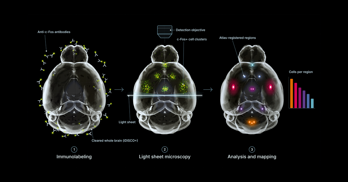
Quantifying c-Fos across a whole mouse brain comes down to five linked steps: acquiring data at a resolution that fits the question, aligning each brain with a reference atlas, detecting c-Fos-positive cells in the 3D volume, extracting metrics per brain region and per voxel, and comparing study groups statistically, with quality control at every step. It is the practical follow-up to What Is Whole-Brain c-Fos Mapping?, which covers what c-Fos measures and when to use it. Most of the problems that surface at the end of a study trace back to a decision made earlier in this chain, often before the brains were imaged. This guide walks through each step, what tends to go wrong, and how to validate a pipeline before trusting its output.

1. Start before the microscope

The quantity you want to compare between groups determines how the brains should be imaged. Cell counts need a resolution and z-step fine enough to separate neighbouring nuclei. If either is too coarse, cells that sit close together merge into one object, and no amount of downstream analysis can split them again. Intensity or coverage measurements are more forgiving.

"Before even starting this whole experiment, you need to know what you want to get out of it, to then know what settings to use for imaging. Every time you make a decision, it's a trade-off on something."

Johanna Perens, CTO, Vibraint

The practical default is the lowest resolution that still answers the question, because data volume grows quickly. One mouse brain at 5 µm isotropic resolution with several channels is typically 20 to 40 GB, while the cellular-resolution scans used for c-Fos cell counting produce hundreds of gigabytes to around 1 TB of raw data per brain. Study design matters here too: for group comparisons we recommend at least eight animals per group. Six per group is workable, but the reduced statistical power should be stated when the results are reported.

2. Preprocess with restraint

Light sheet microscopes acquire data in tiles, so the first step is stitching, often handled by the microscope software. Downsampling to the working resolution usually follows. Further corrections such as de-striping (removing stripe artifacts from the light sheet) or deconvolution (reducing the elongation of signal along the z-axis) are available, but each one changes the signal being measured.

"The more operations you do on your image, the more you also modify the signal. It's very important to be aware of what you're measuring to know what kind of post-processing steps are okay to make."

Johanna Perens

Before analysis starts, every sample is also rotated into a standard orientation, which makes registration more robust and quality control easier to compare across brains.

3. Align brain and atlas, in both directions

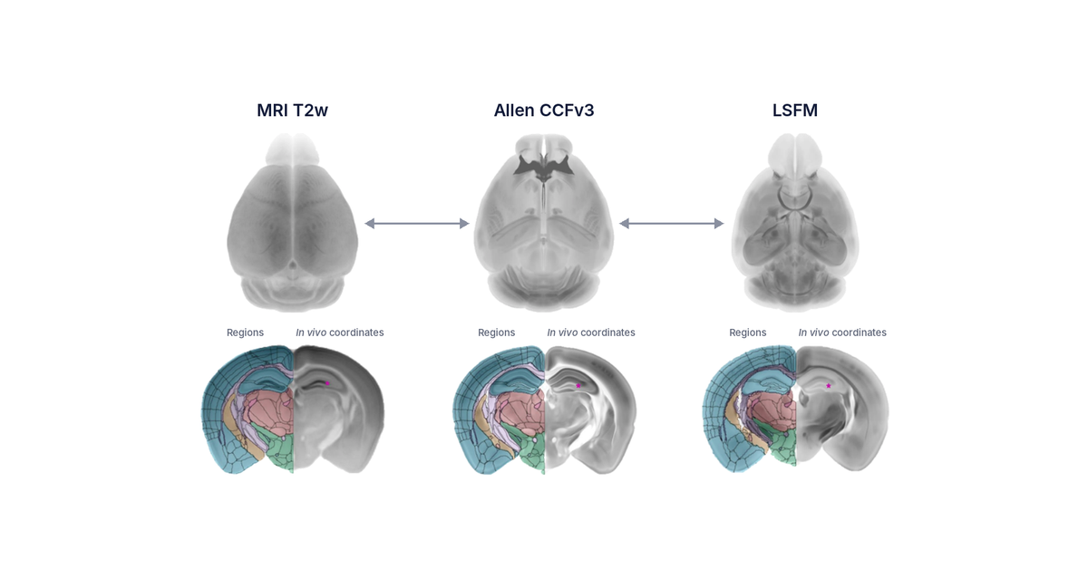
Brain anatomy is highly conserved within a species and strain, which is what makes atlas-based analysis possible. Registration aligns each sample to the reference atlas and the atlas to each sample, producing transformation matrices that move data either way. Both directions are needed: region-wise counting happens in the sample's own space, while group statistics happen in atlas space (see steps 5 and 6).

Vibraint registers to the Perens CCF, a peer-reviewed reference brain built from intact, iDISCO+-cleared mouse brains imaged by light sheet microscopy (Perens et al. 2021, Neuroinformatics), using the established elastix registration toolbox. Registration is very reliable when samples are processed the same way as the brains the template was built from. It becomes less reliable when they differ:

• Sex, age and strain. The template was built from male mice. Female, older, younger or other-strain brains differ subtly in shape.
• Tissue processing protocol. Brains processed with a different clearing or labelling protocol look different. In situ hybridization samples, for example, need their own template.
• Sample integrity. Missing pieces, cuts, and even how much of the brainstem was removed change how the brain deforms.

Often one region of interest maps well while others map less well, which may be acceptable for the question at hand. Automated registration QC flags these cases, and it works best when it is known in advance where the signal is expected. Deep learning registration methods are a promising route to faster and more accurate alignment; in Johanna's tests so far they have matched elastix but not outperformed it, which makes them worth re-testing as new models are published. The atlas comparison is covered in more depth in Choosing a Brain Atlas That Matches Your Method.

4. Detect c-Fos-positive cells

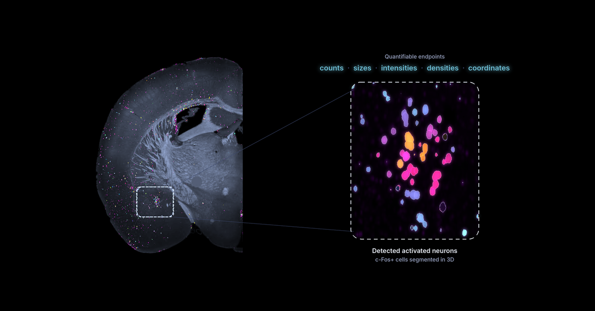
c-Fos is a nuclear marker, which makes it one of the more tractable signals to segment: cells appear as compact, roughly spherical objects. Cytoplasmic markers such as tyrosine hydroxylase are harder, because labelled processes make individual cells difficult to separate. Even so, the segmentation method is chosen and tuned for each study before the high-throughput run begins, using either classical algorithms with tuned parameters, deep learning models fine-tuned to the data, or a combination of both.

Intensity-based pixel classifiers reach a useful starting point but plateau. In Vibraint's pipeline, classical and machine-learning methods produce first-pass segmentations, which are refined manually and then used as ground truth to train deep learning models. The advantage of deep learning here is context: the same c-Fos stain looks different in regions where cells are densely packed compared with sparse regions, and a trained model learns this, along with how to handle the imaging artifacts every scan contains.

Variability is the central difficulty. Microscopes drift over time, lasers fade, staining batches differ, and different microscope architectures produce different artifacts. There is currently no foundation model for light sheet data, so each new dataset is checked against the range of signal and artifact variation seen before, and the model is fine-tuned when the new data fall outside it.

"I don't believe in high-throughput pipelines that don't do any QC, because if you don't check what comes out of your pipeline, you don't actually know if you found all the cells."

Johanna Perens

5. Quantify region by region

For region-wise analysis, the atlas regions are transformed onto each sample, and the chosen metric is extracted for every region, 800+ in the Perens CCF. Across a study this gives a per-region value for each animal, the variance within each group, and statistical tests between groups. Hand-counting at this scale is not realistic, which is why this step is automated.

The standard metrics are:

• Counts of detected cells per region.
• Density, cells per unit volume. Raw counts scale with region size, so density is the fairer figure for comparing regions of different volume.
• Coverage, the fraction of a region's area covered by signal.
• Intensity, summed, mean or median signal per region, the usual readout for fluorescently labelled drug biodistribution.
• Spatial relationships, such as the distance of detected objects to blood vessels.

For c-Fos, counts and densities are the standard readouts, compared against a control group to separate the treatment effect from baseline activation. The choice of metric deserves as much thought as the imaging. Microglia illustrate why: in inflamed tissue they cluster and change shape, and in Vibraint's experience a painstaking per-cell count often shows no change in a region while local density changes substantially.

"Very often scientists come and say, I want it all, all the metrics. But very few of the metrics actually make sense. It's an evolution of understanding what is a reasonable metric to evaluate."

Johanna Perens

6. Compare groups voxel by voxel

Atlas regions are anatomical conventions, and activation does not always respect their borders. Voxel-wise analysis addresses this. Detected cells from each brain are transferred to the atlas resolution without losing information and mapped into atlas space, where animals and treatment groups can be compared directly. The outputs are average heatmaps per group, voxel-wise p-value maps, and maps of signal that is shared or different between groups. Region-wise and voxel-wise analysis complement each other: the first gives numbers per named structure, the second shows where within or across structures an effect sits.

7. Common pitfalls that distort whole-brain c-Fos data

• Acquisition settings that do not match the metric, especially a resolution or z-step too coarse to separate clustered cells.
• Batch effects between staining rounds, and drift between imaging sessions on the same microscope.
• Machine-specific artifacts that differ between microscopes and can be misread as regional effects if not checked against the raw images.
• Over-processing, where correction steps alter the signal being measured.
• Registration mismatch when sex, age, strain, protocol or sample integrity differ from the template.
• Inconsistent perfusion or fixation timing, and time-of-day and handling-stress effects on baseline c-Fos expression, unrelated to the experimental manipulation.

8. Validate the pipeline before trusting the results

Quality control runs through the whole pipeline rather than sitting at the end. The data are checked on arrival for resolution and quality. Segmentation is checked against manually annotated ground truth in representative regions and brains. Registration is checked both automatically and visually against known landmarks. Whether the pipeline runs in-house or with a provider, the same questions apply: what was checked at each step, and can the validation data be shown on request.

9. What the output looks like

The figure below shows the two outputs side by side for semaglutide-treated mice compared with vehicle-treated controls. On the left is the group average c-Fos heatmap in atlas space, the voxel-wise view from step 6. On the right is the region-wise result from step 5: for each brain region, the log₂ fold change in mean c-Fos density between the two groups, ordered by major brain division from cerebrum to cerebellum.

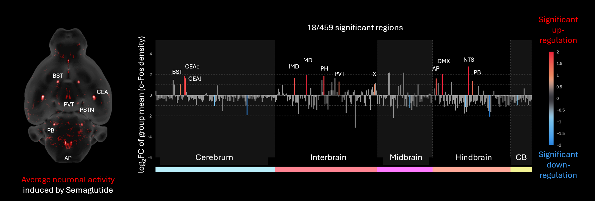
Whole-brain c-Fos response to semaglutide. Left: average neuronal activity induced by semaglutide, horizontal view. Right: log₂ fold change of group mean c-Fos density per region versus vehicle; 18 of 459 regions were significant. Red bars mark significant increases, blue bars significant decreases, grey bars non-significant changes.

Of the 459 regions tested in this analysis, 18 changed significantly. The increases form a recognisable circuit: in the hindbrain, the area postrema (AP), nucleus of the solitary tract (NTS), dorsal motor nucleus of the vagus (DMX) and parabrachial nucleus (PB); in the interbrain, the paraventricular thalamic nucleus (PVT), mediodorsal (MD) and intermediodorsal (IMD) thalamic nuclei, posterior hypothalamus (PH) and the xiphoid thalamic nucleus (Xi); and in the cerebrum, the bed nucleus of the stria terminalis (BST) and the capsular and lateral parts of the central amygdala (CEAc, CEAl). The NTS shows the largest increase. Significant decreases are fewer and smaller.

Two points from earlier sections show up directly in this result. The metric is density compared against a control group, not raw counts, so regions of very different size can be ranked on one axis. And because every region is tested, the figure also shows what did not change, which is as informative for interpreting a mechanism as the handful of regions that did. Results like these, including the 3D position of every detected cell, can be explored region by region on CNS-Voyager™, and the biology behind the pattern is discussed in our post on how semaglutide affects the brain.

With 800+ regions available and far more voxels, the harder problem is exploring results like these without cherry-picking a few favourite regions. That is why Vibraint delivers results in CNS-Voyager™, a browser-based 3D and 2D brain viewer where all maps sit in atlas space, every region can be inspected, and coordinates of interesting signal can be read off for follow-up experiments. Individual detected cells can also be inspected, with per-object properties such as intensity, size and sphericity.

10. Going further with the same data

Per-region c-Fos values across a cohort are a starting point for further analysis. Correlated activity across animals supports functional connectivity analysis, and graph-based methods can describe how activated regions relate to each other as a network. Integrating the activity maps with other datasets in the same atlas space, such as gene expression maps, helps narrow down which cell types sit in an activated region. These analyses are not standard in every pipeline, and which one fits depends on the scientific question.

11. Build, buy, or bring your own data

• Do it yourself with open tools such as BrainGlobe or ClearMap. This is a legitimate path for a lab with computational support and time to validate its own pipeline. Vibraint also offers consulting to labs that want to run the analysis themselves.
• Run the full pipeline through LS-Journey™: whole-brain immunolabeling, light sheet imaging and image analysis, registered to the Perens CCF and delivered on CNS-Voyager™.
• Bring your own light sheet data for analysis only. This route suits academic, biotech and pharma groups that already have a light sheet microscope and the wet-lab skills, but no image analyst specialized in brain data. Standard TIFF and HDF5 output works with the pipeline, and data are uploaded to a dedicated cloud bucket with upload guidelines. The analysis runs on Vibraint's own Python pipelines and servers.

Whichever route fits, the most useful moment to discuss analysis is before imaging, when the metric, resolution and group size can still be chosen to match the question.

Frequently asked questions

How do you quantify c-Fos across the whole mouse brain?

Whole-brain c-Fos quantification involves acquiring light sheet data at a resolution suited to the question, aligning each brain with a reference atlas, detecting c-Fos-positive cells in the 3D volume, extracting counts and densities for every atlas region, and comparing study groups region by region and voxel by voxel. Each step needs quality control, including checking automated cell detection against manually annotated ground truth.

Can you manually count c-Fos-positive cells across an entire mouse brain?

Manually counting across all 800-plus regions of a reference atlas, for every brain in a study, is not a realistic workflow. Whole-brain quantification is therefore automated, while manual counting remains essential as ground truth for training and validating the automated detection.

What is the difference between raw cell counts and density when quantifying c-Fos?

Raw counts per brain region scale with region volume, so a larger region contains more cells even with no difference in activation. Density, cells per unit volume, corrects for this and is the fairer figure for comparing regions of different sizes. Comparing either metric against a control group separates the treatment effect from baseline activation.

What causes inaccurate results in whole-brain c-Fos quantification?

Common sources of error include imaging at a resolution or z-step too coarse to separate clustered cells, batch effects between staining or imaging sessions, microscope-specific artifacts, over-processing of images, registration mismatch when sex, age, strain or tissue protocol differ from the atlas template, inconsistent perfusion or fixation, and baseline c-Fos changes from time of day or handling stress.

How many animals per group do you need for a whole-brain c-Fos study?

Vibraint recommends at least eight animals per group for statistical group comparisons. Studies with six animals per group are possible, but the reduced statistical power should be noted when the results are reported.

Can Vibraint analyze light sheet data acquired in my own lab?

Yes. The image analysis module of LS-Journey™ is available on its own for externally acquired light sheet data. Standard TIFF and HDF5 formats work with the pipeline, and data are shared via a dedicated cloud bucket. A scoping meeting comes first, ideally before imaging, so that acquisition settings match the metrics to be quantified.

How long does whole-brain c-Fos analysis take?

A full-pipeline study typically takes two to two and a half months from sample receipt to data delivery. Whole-brain immunolabeling takes about a month regardless of the number of brains, because antibodies need time to penetrate the intact tissue evenly. Imaging a c-Fos brain realistically takes one to two hours including remounting, depending on resolution and signal intensity, and can be shorter or longer for other markers. Automated analysis and atlas registration follow.

Plan your whole-brain c-Fos analysis

The metric, resolution and group size are easiest to get right before the first brain is imaged. We start every study, including analysis-only projects, with a scoping discussion. Read about AI-assisted image analysis, explore LS-Journey™ or explore whole-brain data on CNS-Voyager™.

References

1. Perens J, Salinas CG, Skytte JL, et al. An optimized mouse brain atlas for automated mapping and quantification of neuronal activity using iDISCO+ and light sheet fluorescence microscopy. Neuroinformatics 2021;19:433-446. doi:10.1007/s12021-020-09490-8
2. Renier N, Adams EL, Kirst C, et al. Mapping of brain activity by automated volume analysis of immediate early genes. Cell 2016;165(7):1789-1802. doi:10.1016/j.cell.2016.05.007
3. Klein S, Staring M, Murphy K, Viergever MA, Pluim JPW. elastix: a toolbox for intensity-based medical image registration. IEEE Transactions on Medical Imaging 2010;29(1):196-205. doi:10.1109/TMI.2009.2035616
4. Wang Q, Ding SL, Li Y, et al. The Allen Mouse Brain Common Coordinate Framework: a 3D reference atlas. Cell 2020;181(4):936-953. doi:10.1016/j.cell.2020.04.007